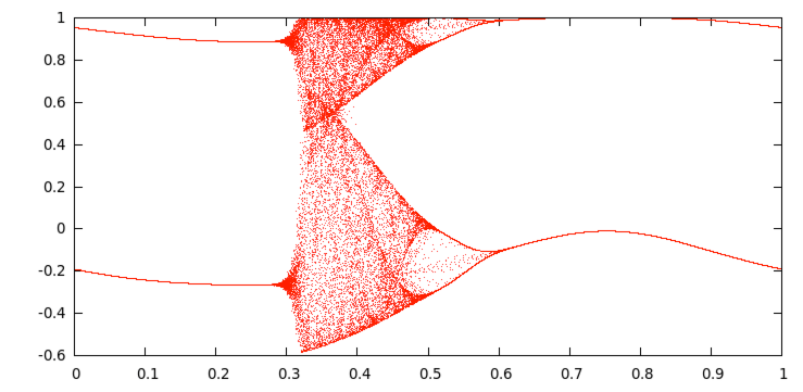
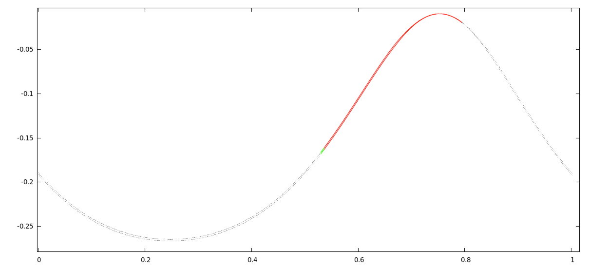
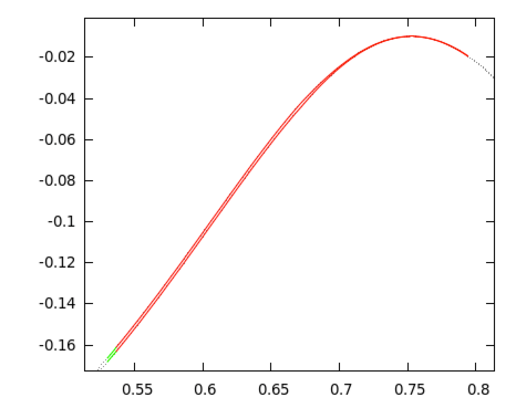
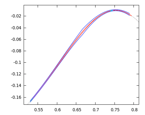
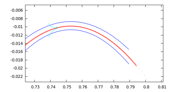
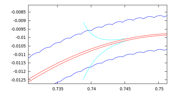
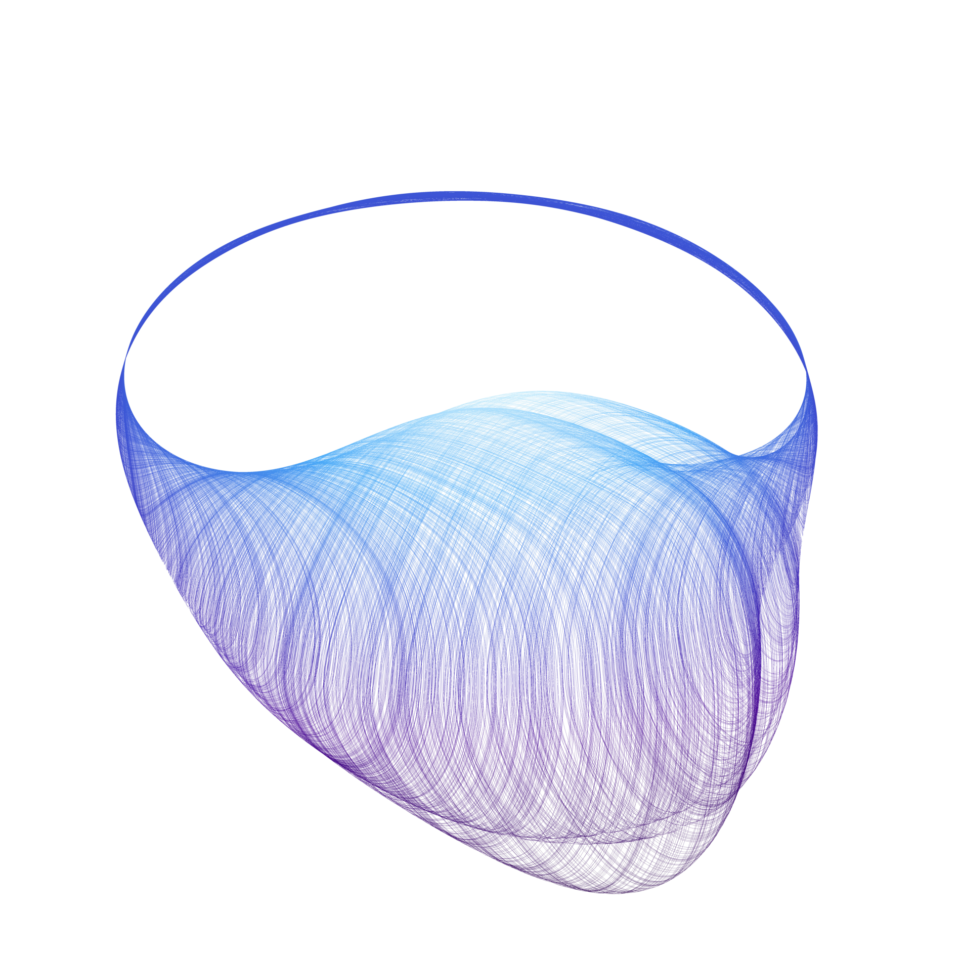
Can one blindly believe numerical simulations? I think that we all know the answer to this. In some cases "numerical evidence" might be very mistakingly interpreted. An example of this is a simple driven logistic map

T : 𝓢¹⨯ℝ →𝓢¹⨯ℝ,
T(θ,x) =(θ+α,1-(a+ε sin(2πθ))x²),

with a=1.31, ε=0.3 and α=g/200, where g is the golden mean g=0.5(√5-1). The map possesses a global attractor, but when standard (double precision) numerical simulation is performed, this attractor seems to be chaotic. This is not the case. When redoing the computations with multiple precision we find that this attractor is in fact composed of two smooth curves. With the CAPD package we have proved that this is the case.

The two curves are normally hyperbolic invariant manifolds. In some parts they are strongly contracting, but in many parts they are expanding. Since the map is nasty enough to mislead standard non-rigorous simulations, in our proof we needed to consider multiple precision (tracking 40 digits), combined with 𝓒¹⁰ methods. The proof is based on covering relations combined with cone conditions.

This description by Maciej Capinski.

• Maciej Capinski and Carles Simó, Computer Assisted Proof for Normally Hyperbolic Invariant Manifolds, Nonlinearity 25 (2012), no. 7, 1997-2026.

Misleading numerical plot of the attractor.

Our rigorous estimate of the attractor for T².

Sets and covering relations used in our proof.

In bright blue, a covering which involves 128 iterates a local inverse map of T².